


Linear Programming and the Simplex Algorithm
A hopefully comprehensive FAQ

This post is a summary of my leanings about the simplex algorithm. I’ve tried to focus on providing intuition for the why the algorithm works as opposed to the how, by making lots of analogies to geometry.
For context, my fourth year ECE532 course involves a semester-long group project with the task of implementing something cool on an FPGA (a type of re-programmable computer chip). My team is attempting to implement the simplex algorithm on an FPGA for power modelling applications.
I don’t expect most of the content to be interesting or relevant to most readers, but I’ll be happy if it is to some.
Table of Contents
What is linear programming?
Linear programming is an approach to solving constrained linear optimization problems. Let’s break that down.
Optimization problems try to find the maximum or minimum value. They are used to answer question like, “how can I maximize my revenue” or “how should I operate this electricity grid to minimize costs.” Formally, we say that optimization problems minimize or maximize an objective function.
A constrained optimization problem means that there are hard limits on the range of acceptable solutions. For example, “I want to find the minimum solution but my variable x has to be greater than 4.” Or more concretely, “How should I operate this electricity grid to minimize costs assuming my nuclear power plant needs to always generate at least 4 MW?”

A linear constrained optimization problem means that both the objective and the constraints are linear functions. Linear optimization is a subset of the well-studied field of convex optimization.

How is linear programming used in power systems?
Linear programming is central to how we plan our electricity grids. Let’s look at a toy example.
We have two small towns, CleanVille and DirtyVille.
Each town needs 100 MW of power.
CleanVille has a hydro plant that can generate up to 190 MW at $30 per MW.
DirtyVille B has a gas plant that can generate up to 200 MW at $50 per MW.
The two towns are connected by a transmission line that can carry up to 80 MW.What’s the most cost-effective way to operate the electricity grid?
We can use linear programming to solve this problem! First we create our linear program as shown below. This linear program is expressing our problem as a linear objective function with a set of linear constraints. Note that our linear program has 3 variables: x, y, z.

Note that every linear program is a model of reality. For example, here we’ve chosen not to account for transmission losses. Does that mean our model is wrong? Yes, but that’s ok. Remember: “all models are wrong, but some are useful.”
How do we solve a linear program?
In practice you use a solver. These are existing libraries that solve linear programs for you. If you’re in academia or you’re a rich business you use Gurobi, the leading commercial solver. Otherwise, you can use an open-source solver like HiGHS.
But what do these solvers actually do? There are two algorithms to solving linear programs: the simplex method and interior-point method. Each method has different variations too.

I do not discuss the interior-point method in this post but this video does an outstanding job at explaining it.
The Simplex Algorithm
This video gives an outstanding overview of the simplex algorithm. I recommend watching it. Here’s my attempt at explaining the simplex algorithm.
How does the simplex algorithm work conceptually?
Consider an optimization problem with just two variables as shown below.
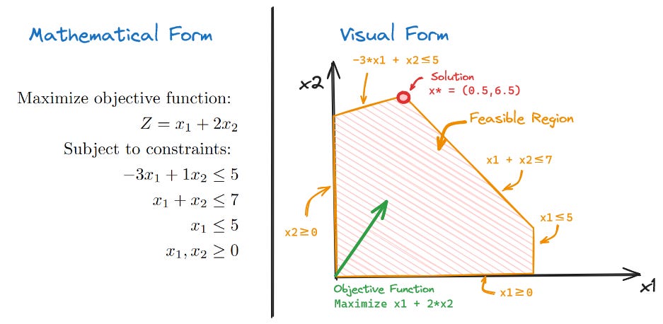
The mathematical form and visual form are completely equivalent. The visual form of the optimization problem is asking, if we are pushed in the direction of the objective function (green arrow) and we must stay in the feasible region (orange boundaries) where do we end up? We quickly see that we end up at the corner marked in red. This is the optimal solution.
If this is confusing, consider that moving perpendicular to the green objective arrow (along the thin red lines) has no cost since the objective doesn’t change (the red lines are the objective function’s ‘level set’). All we care about is moving as much as possible in a direction parallel to the green arrow.
Intuitively, you might guess that the optimal solution is always at a corner. This turns out to be true!1 This concept can be generalized to higher dimensions. Edges become planes (or hyperplanes), corners become vertices, and polygons become polytopes. Still, optimal solutions always lie on corners (vertices). We can say, for a problem with n variables, the solution is always at the intersection of n constraints since a vertex is just an intersection of n constraints. I will continue to use the corner and edge terminology, but know that we are really talking about vertices and hyperplanes.
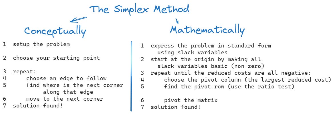
So, how does the simplex algorithm work conceptually? Well, the simplex algorithm moves from corner to corner, always in the direction of the objective, until it eventually reaches the ‘furthest’ corner and cannot go further—it has found the solution.
How does standard simplex work mathematically?
Here’s a mapping of the conceptual steps in the simplex algorithm to the mathematical steps.
The diagram below shows the process for solving an example linear program using the standard simplex method. I’ll dive into each step and hopefully give you some intuition of why the algorithm works.

First, to understand the simplex method we must formalize the meaning of “moving from corner to corner” which requires formalizing the meaning of “being at a corner.”
Recall, we are at a corner when we are on the ‘edge’ of n different constraints where n is the number of variables. But what does it mean mathematically to be on the edge of a constraint?
We are on the edge of a ≤ constraint when the LHS = RHS rather than the LHS < RHS. We can express this mathematical by introducing a “slack variable” as shown below. We the slack variable is zero, we must be on the edge of the constraint.
Now I’ve rewritten the linear program in matrix form with slack variables. We call this “standard form.”

Notice if we set any variable to zero, we must be on an edge. If x₁ or x₂ is set to zero, we must be on the x₁≥0 or x₂≥0 edge. If a slack variable is zero we must be on that constraint’s edge as mentioned earlier. We start our algorithm by setting all x variables to zero, effectively placing us at the origin.
Therefore, if n variables are zero, we are at a corner. Hence, to move from one corner to another, we must set one variable to zero in exchange for ‘unsetting’ one variable from zero. This effectively ‘swaps’ or ‘pivots’ a variable which moves us to a neighbouring corner. Variables that are set to zero are called non-basic while variables that aren’t are basic variables.
Naturally, this raises two questions:
On each ‘pivot,’ which variable do we unset from zero (move into the basis)?
On each ‘pivot,’ which variable do we set to zero (remove from the basis)?
The answer to these questions is as follows.
The simplest approach is to use the Dantzig rule which says that we unset whichever variable has the largest ‘reduced costs.’ Reduced costs is a measure of how much the objective function will increase when we unset our variable from zero. The more it increases, the faster we will maximize our objective. The reduced costs are simply the coefficients in the objective when the objective is expressed only in terms of the non-basic variables. I found this explanation quite helpful.
We set to zero whichever variable we encounter ‘first.’ What does this mean?
Geometrically ‘unsetting’ a variable from zero is ‘unlocking’ us. Previously we were locked to the corner, but now we can move away from it along an edge towards the next corner. The moment we encounter a new corner we must stop and fix ourselves to it. This is because, if we go beyond this ‘first’ corner we will exist the feasible region. Therefore, we want to find the first constraint that intersects our edge since that point of intersection will be the first corner. Mathematically, this is done using the ratio test. Basically, the ratio test asks, “If all the basic variables (variables that we might want to set to zero) were already at zero, what value would the variable entering the basis (the variable we’ve just unset from zero) take on?” The smallest positive answer to this question tells which basic variable becomes zero first. This variable corresponds to our pivot row and destination corner. The ratio test is shown below.
The calculation above was rather simple because we only needed to divide two numbers and find the minimum. However, this was only possible because the matrix values for the unlocked (basic) variables were unit vectors. To preserve this property, we must perform a pivot using row operations after every iteration. Here’s the pivot on this step.
Notice how now the matrix columns corresponding to non-zero variables x₂, s₁, and, s₂ are still unit vectors. The pivot worked!
We repeat the process, unlocking x₁, in exchange for locking s₂ (since 2/4 is the smallest non-negative ratio in the entries of the RHS divided by the pivot column). The result after performing the pivot is:
From here, we easily see that x₁=0.5 and x₂=6.5 (since s₁ and s₂ are non-basic and set to zero). We’ve solved our problem.
How do we get a linear program into standard form?
An important point I’ve purposely ignored up to now is, how does one get a linear program into standard form? We discussed adding slack variables, however, this is not sufficient. Particularly, standard form requires:
all x variables are non-negative
all slack variables are non-negative
the RHS b values are non-negative
it’s a maximization problem (not minimization)
So how do we express constraints like -∞≤x≤5 or x+y≥1? There exists a variety of tricks to do this.
Even these tricks are sometimes insufficient. If the linear program includes a constraint like x + y ≥ 1 then the origin is not a feasible solution so it would be impossible to use our algorithm (our algorithm is expected to start at the origin!). Instead, we need to solve an easier optimization problem to find a starting point, before then proceeding to solve the original problem.
Conclusion
There is so much more I’d love to share about linear programming including details on its practical uses in modelling electricity grids (see my paper on the topic!) or the different performance and memory tradeoffs between various solving algorithms (leveraging sparsity is cool!). Unfortunately, those will have to wait for another time.
There is a special case where the ‘last’ edge is exactly perpendicular (normal) to our objective function. In this case, any point on that edge is optimal—there exists multiple optimal solutions. Nonetheless, one of the many optimal solutions is right where the edge meets another edge. That’s to say, there is some optimal solution at a corner.